Lynn Le | Blogpost5| Reinforcement learning: Policy-based

Bological entities can extract a large amount of information from binary feedback signals. Reinforcement learning (RL) is a general term for an agent that learns to act using reinforce signals (for example reward or punishment). Two important types of RL in machine learning are Deep Q-learning and policy-based RL. This post is focused on the latter.

An agent that does policy-based RL, learns by updating the parameters of its policy π, which is based on the state that the agent is in and its received reward upon performing an action.

In machine learning, the π can be seen as a differentiable function, which can be implemented with a neural network. The π receives a state as an input and in return outputs different probability scores of each action. In this post, I will focus on explaining how we can use this policy network to perform reinforcement learning.

The environment

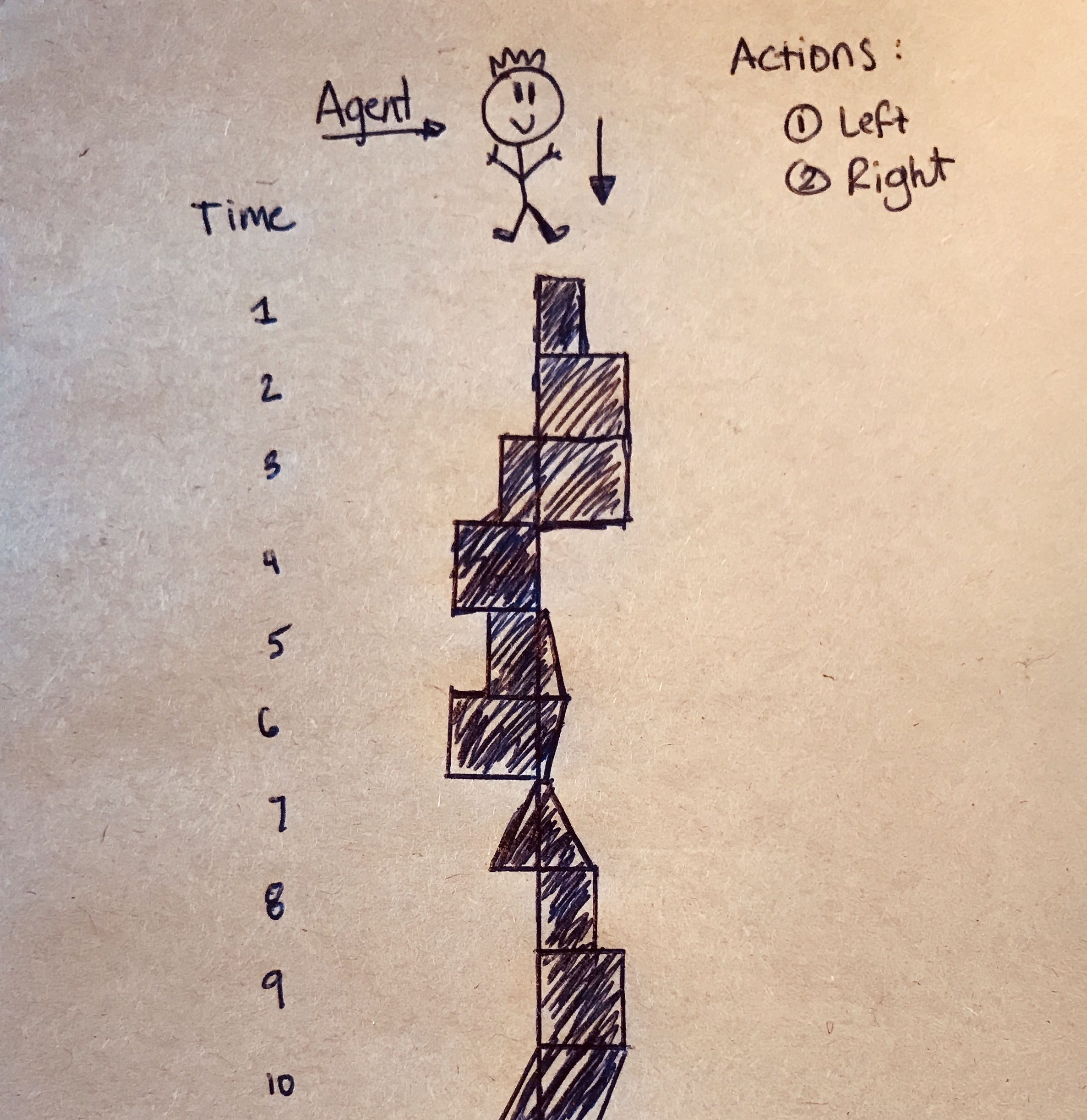
Imagine an agent running down a continous plateau with the aim to stay on the plateau as long as possible. At every timestep t, he encounters a different surrounding structure and needs to decide whether to shift himself to the right or left in order to stay “alive”. His lifespan is represented as (t₁, …, T). The longer he manages to survive during his run, the better his performance.

Some definitions (in our environment)

Agent: The agent interacts with its environment by performing actions in discrete time steps.
Actions a_t : The action that the agent can take at timestep t. At each timestep, the agent can either shift to the left, or to the right.
State s_t: The state that the agent is in at timestep t.
Reward r_t: The reward returned at timestep t.
Episode: Everytime the agent runs on the plateau to learn, it creates an episode that contains all the actions taken at every timestep.
Policy π : Is the basic neural network that predicts the probability scores of every action at each time step given a state.

The learning concept

Basically, the reinforcement algorithm is represented by the following equation:

$\nabla J(\theta) = \frac{1}{N}\sum_{i=1}^N\Big({\sum_{t=1}^T}{\nabla_\theta \log{\pi_\theta}(a_{i,t}|s_{i,t})}\Big) \Big(\sum_{t=i}^T r(s_{i,t}, a_{i,t})\Big)$

Where r(s_i,t,a_i,t) is the reward at (s_i,t,a_i,t).

During each episode, the agent runs on the plateau and performs some actions. After the episode, we make use of the reinforce algorithm to update the parameters of the policy network and then run it again.

In other words, we want to optimize the parameters in such a way that maximizes the gradient of θ. This is done in three steps:

Run the policy network π_θ(a_t|s_t) which outputs various action probability scores (τ) given a state s_t and sample a probability score τⁱ from the output.
Then, we want to calculate the gradient ascent:

$\nabla J (\theta) \approx \sum_i \Big( \sum_t \nabla_\theta \log\pi_\theta(a_{i,t} | s_{i,t}) \Big) \Big(\sum_t r(s_{i,t}, a_{i,t})\Big)$

To ultimately update the parameters of the policy network:

$\theta \leftarrow \theta + \eta \nabla_ \theta J(\theta)$

Using cost to go to reduce variance

So far I have explained the basic reinforcement algorithm. This explained algorithm learns by using ALL the rewards that it gets during that entire episode. Since the π_t’ cannot affect the rewards that occurred before t, it results in a high variance method of learning.

To reduce the variance, we can make use of the future rewards after an action is performed, such that the agent performs based on future rewards only.

This means that the reinforce algorithm becomes:

$\nabla J (\theta) = \frac{1}{N}\sum_{i=1}^N \sum_{t=1}^T \nabla_\theta \log\pi_\theta(a_{i,t} | s_{i,t})\hat{Q}_{i,t}$

Where the Q-hat is the ‘cost-to-go’:

$\hat{Q}_{i,t} = \sum_{t' = t}^T r(s_{i,t'}, a_{i,t'})$

which is the collection of all the future rewards, after a performed action at t.

To summarize

For each episode, the agent gets to run on the plateau. For each timestep in the episode, the policy takes in a state, and outputs different probabilities of actions, and one action is then randomly sampled (the actions with higher probability scores have a higher probability to be sampled). This happens until the agent falls off the plateau.

We then look at each timestep of that episode, starting at the first timestep. At the first timestep, we sum all the rewards following that timestep, and then update the policy parameters of that timestep, such that the policy output has a positive effect on the total future reward (this we call gradient ascend).

Then for the next timestep of that same episode, we again sum its future rewards, and again the parameters of the policy network is updated based on that sum. When repeating this with many episodes, the policy output becomes more optimal at each timestep and the episodes become longer.

Reference

I have learned all of this material in the Neural Information Processing Systems course, this year!