Hi! I made a simple game using Unity and C#. To start playing it, please press enter :D

Bological entities can extract a large amount of information from binary feedback signals. Reinforcement learning (RL) is a general term for an agent that learns to act using reinforce signals (for example reward or punishment). Two important types of RL in machine learning are Deep Q-learning and policy-based RL. This post is focused on the latter.

An agent that does policy-based RL, learns by updating the parameters of its policy π, which is based on the state that the agent is in and its received reward upon performing an action.

In machine learning, the π can be seen as a differentiable function, which can be implemented with a neural network. The π receives a state as an input and in return outputs different probability scores of each action. In this post, I will focus on explaining how we can use this policy network to perform reinforcement learning.

The environment

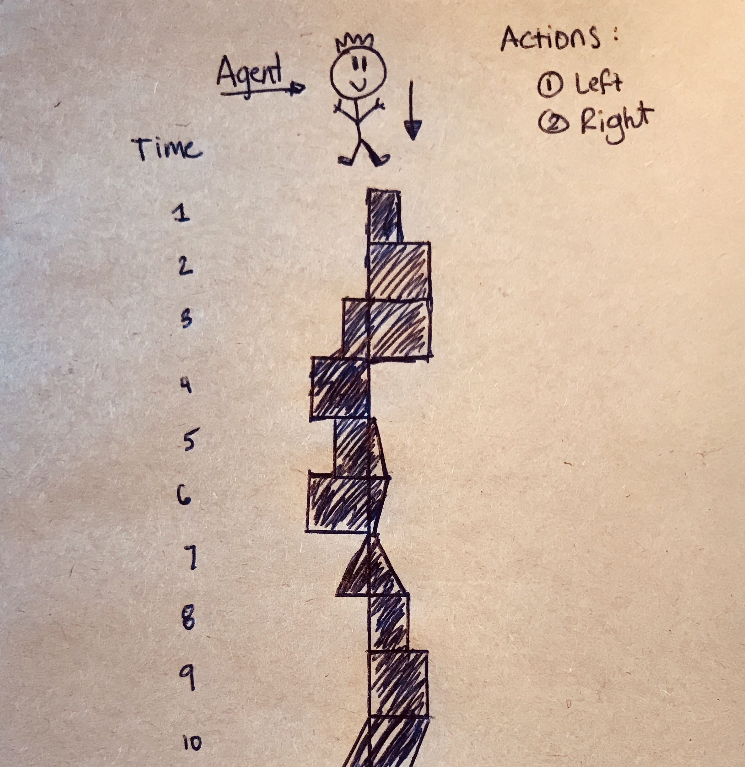
Imagine an agent running down a continous plateau with the aim to stay on the plateau as long as possible. At every timestep t, he encounters a different surrounding structure and needs to decide whether to shift himself to the right or left in order to stay “alive”. His lifespan is represented as (t₁, …, T). The longer he manages to survive during his run, the better his performance.

Some definitions (in our environment)

• Agent: The agent interacts with its environment by performing actions in discrete time steps.
• Actions a_t : The action that the agent can take at timestep t. At each timestep, the agent can either shift to the left, or to the right.
• State s_t: The state that the agent is in at timestep t.
• Reward r_t: The reward returned at timestep t.
• Episode: Everytime the agent runs on the plateau to learn, it creates an episode that contains all the actions taken at every timestep.
• Policy π : Is the basic neural network that predicts the probability scores of every action at each time step given a state.

The learning concept

Basically, the reinforcement algorithm is represented by the following equation:

Where r(s_i,t,a_i,t) is the reward at (s_i,t,a_i,t).

During each episode, the agent runs on the plateau and performs some actions. After the episode, we make use of the reinforce algorithm to update the parameters of the policy network and then run it again.

In other words, we want to optimize the parameters in such a way that maximizes the gradient of θ. This is done in three steps:

1. Run the policy network π_θ(a_t|s_t) which outputs various action probability scores (τ) given a state s_t and sample a probability score τⁱ from the output.

2. Then, we want to calculate the gradient ascent:

1. To ultimately update the parameters of the policy network:

Using cost to go to reduce variance

So far I have explained the basic reinforcement algorithm. This explained algorithm learns by using ALL the rewards that it gets during that entire episode. Since the π_t’ cannot affect the rewards that occurred before t, it results in a high variance method of learning.

To reduce the variance, we can make use of the future rewards after an action is performed, such that the agent performs based on future rewards only.

This means that the reinforce algorithm becomes:

Where the Q-hat is the ‘cost-to-go’:

which is the collection of all the future rewards, after a performed action at t.

To summarize

For each episode, the agent gets to run on the plateau. For each timestep in the episode, the policy takes in a state, and outputs different probabilities of actions, and one action is then randomly sampled (the actions with higher probability scores have a higher probability to be sampled). This happens until the agent falls off the plateau.

We then look at each timestep of that episode, starting at the first timestep. At the first timestep, we sum all the rewards following that timestep, and then update the policy parameters of that timestep, such that the policy output has a positive effect on the total future reward (this we call gradient ascend).

Then for the next timestep of that same episode, we again sum its future rewards, and again the parameters of the policy network is updated based on that sum. When repeating this with many episodes, the policy output becomes more optimal at each timestep and the episodes become longer.

Reference

I have learned all of this material in the Neural Information Processing Systems course, this year!

Trained models

The pretrained models that I used (models provided by PyTorch) all contained linear layers as last layers. I replaced these layers with convolutional layers since I do not want to loose spatial information when predicting my outputs. Additionally I had a self-made deep neural network which consisted of residual blocks and deconvolution layers. I then trained the models separately and ended up having 7 models that performed well.

Ensembling the models

In order to make a supermodel in PyTorch, we first have to make instances of every model classes. Since we have 7 quite large models, I made a separate file containing all the model classes, and named in all7models.py. First I need to import all necessary things:

import torch.nn as nn
import torchvision.models as models
import torch
import torch.nn.functional as F
import numpy as np

Then all the different classes of models that were trained. Here is ana exmaple of the AlexNet model (1 out of 7):

#   ::::::::::::::::::::::::::::::::::::::::::::::::::::::::::::::::::::::::::::::::::::::::::
#   :   A l e x N e t                                                                        
#   ::::::::::::::::::::::::::::::::::::::::::::::::::::::::::::::::::::::::::::::::::::::::::
class AlexNet(nn.Module):
    def __init__(self, outsize):
        super(AlexNet, self).__init__()
        self.outsize = outsize
        self.alexnet = models.alexnet(pretrained = True)
        self.convout = nn.Sequential(
            nn.Upsample(48),
            nn.Conv2d(in_channels=192, out_channels=192, kernel_size=3, stride=1, padding=1),
            nn.BatchNorm2d(192),
            nn.ReLU(),
            nn.Upsample(48),
            nn.Conv2d(in_channels=192, out_channels=96, kernel_size=3, stride= 1, padding=1),
            nn.BatchNorm2d(96),
            nn.ReLU(),
            nn.Upsample((self.outsize[0]+3, self.outsize[1]+3)),
            nn.Conv2d(in_channels=96, out_channels=1, kernel_size=6, stride= 1, padding=1)
            )

    def forward(self, x):
        x = self.alexnet.features[:5](x)
        x = self.convout(x)
        y = torch.sigmoid(x)
        return y 

I used the pretrained model from torchvision.models.alexnet(pretrained=True) and then replace the last layers with a sequentual layer containing upsampling, convolutional, batchnormalization and rectified linear unit layers to ultimately obtain an output of my desired dimensions. The layers that were replaced with the sequential layer were selected based on their outsize, meaning I only ended up using pretrained layers that kept the images at large enough dimensions (again, to keep enough spatia information). I did this with every model and found that they predicted nice outputs.

Anyways, when all the instances of the models are made, the instance of the ensemble can be made. This is a class that initializes all the instances of the models. For PyTorch, it is done like this:

class MyFinalEnsemble_cpu(nn.Module):
    def __init__(self, outsize):
        super(MyFinalEnsemble, self).__init__()
        """
        This is the ensemble of the SuperModel that is built up of the models (with some having shorter amount of iterations than 50). 
        The AlexNet 100x, the DenseNet 100x, InceptionV3 100x, ResDeconv 30x, ResNet 100x, SqueezeNet 25x, and VGG 19x."""
        
        self.outsize = outsize
        
        self.alexnet = AlexNet(self.outsize)
        self.alexnet.load_state_dict(torch.load('final_runs_48x64/AlexNet/AlexNet100ep_48x64', map_location='cpu'))
        
        self.densenet = DenseNet201(self.outsize)
        self.densenet.load_state_dict(torch.load('final_runs_48x64/DenseNet201/DenseNet100ep_48x64', map_location='cpu'))
        
        self.inceptionv3 = InceptionV3(self.outsize)
        self.inceptionv3.load_state_dict(torch.load('final_runs_48x64/InceptionV3/InceptionV3_100ep_48x64', map_location='cpu'))
        
        self.resdeconv = ResblocksDeconv(3, self.outsize, self.outsize)
        self.resdeconv.load_state_dict(torch.load('final_runs_48x64/ResDeconv/ResDeconv30ep_48x64', map_location='cpu'))
        
        self.resnet = ResNet152(self.outsize)
        self.resnet.load_state_dict(torch.load('final_runs_48x64/ResNet152/ResNet152_100ep_48x64', map_location='cpu'))
        
        self.squeezenet = SqueezeNet1_1(self.outsize)
        self.squeezenet.load_state_dict(torch.load('final_runs_48x64/SqueezeNet/SqueezeNet25ep_48x64', map_location='cpu'))
        
        self.vgg19 = VGG19BN(self.outsize)
        self.vgg19.load_state_dict(torch.load('final_runs_48x64/VGG19BN/VGG19BN18ep', map_location='cpu'))

        
    def forward(self, x):
        x1 = self.alexnet(x)
        x2 = self.densenet(x)
        x3 = self.inceptionv3(x)
        x4 = self.resdeconv(x)
        x5 = self.resnet(x)
        x6 = self.squeezenet(x)
        x7 = self.vgg19(x)
        
        x = sum([x1, x2, x3, x4, x6])/5

        return x

Initializing the ensemble

So now that the instances of the models and the the final ensemble are made, the all7models.py is complete and ready to be used.

In a separate file (I used a jupyter notebook file) in the same directory, I can do:

import all7models

Then I can initialize the ensemble like this:

model = all7models.MyFinalEnsemble(outsize)
model.eval()
model.cuda(device)

And then the model can be used to predict!!